Interpretability: Why AI Needs to Explain Itself
Machine learning models shouldn't be black boxes. To build trust, explanations must be:
- Human-friendly (think "tumor spotted" vs. "layer 3 activated").
- Meaningful (using real-world concepts like medical anomalies).
While post-hoc tools (e.g., LIME, SHAP) retroactively decode decisions, prototype networks bake clarity into their design by learning recognizable examples (e.g., "typical pneumonia scans") and justifying predictions by similarity to these prototypes.
👉 Dive deeper → XAI Overview
Prototype Networks: What & Why?

A prototype is essentially a "representative example" or "ideal" for a particular class. For instance, if you're building a model to distinguish cats from dogs, the prototype for a "cat" might be an archetypal cat image (e.g., a typical tabby cat face). By referencing these prototypes, the network can make decisions in a way that's much closer to the way humans reason:
"This input looks a lot like this prototype of a cat's face... so I'm leaning towards cat."
Instead of magical black-box numbers, you can see these prototypes directly and understand the model's reasoning process.
Prototypes vs. Prototypical Parts
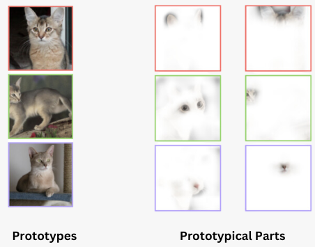
In some prototype-based systems, we talk about prototypical parts. Think of these as smaller or more localized prototypes like specific patches or features within an image. For example:
- Prototype: A full X-ray image representing a certain bone fracture.
- Prototypical Part: The specific region on that X-ray showing the fracture line.
| Aspect | Prototype | Prototypical Parts |
|---|---|---|
| Scope | Whole example or data point (e.g., entire X-ray). | Specific features or regions (e.g., fracture region). |
| Purpose | Offers a global, high-level explanation. | Zooms into local, feature-level details. |
| Interpretability | Compares new inputs to known examples. | Shows which specific parts matter most to the model. |
| Techniques | Prototype-based learning, similarity-based methods. | Concept/feature activation, prototype-part networks. |
| Examples | A typical "cat" image for the "cat" class. | "Cat's whiskers" or "ear" prototypes. |
It's the difference between "Here's the image that convinced me it's a cat" versus "I specifically focused on the whiskers to confirm it's a cat."
Why not just use apply Post hoc methods?
Post-hoc techniques (e.g., saliency maps, Grad-CAM) apply to any model after training, offering flexibility but indirect explanations through approximations like gradients or feature reconstructions. These methods can be noisy and lack inherent transparency. Prototypical networks (e.g., ProtoPNet) bake interpretability into their architecture, learning human-understandable prototypes (e.g., "spotted fur patterns") during training. This ensures direct reasoning but may limit model flexibility. Below, a concise comparison:
| Aspect | Post-hoc Techniques | Prototypical Approach |
|---|---|---|
| Timing | After the model is trained. | Built into training architecture & procedure. |
| Focus | Explains individual decisions or patterns post-training. | Learns prototypes/parts for direct interpretability. |
| Interpretability | Indirect (gradient-based or reconstruction-based). | Direct, from the design of the network. |
| Flexibility | Works with any architecture. | Requires specific design (e.g., ProtoPNet). |
| Examples | Saliency maps, Grad-CAM, Activation Maximization. | Prototype networks (ProtoPNet), concept-based models. |
| Limitations | Can be noisy, not always trustworthy. | Model complexity can be restricted for interpretability. |
ProtoPNet in Detail
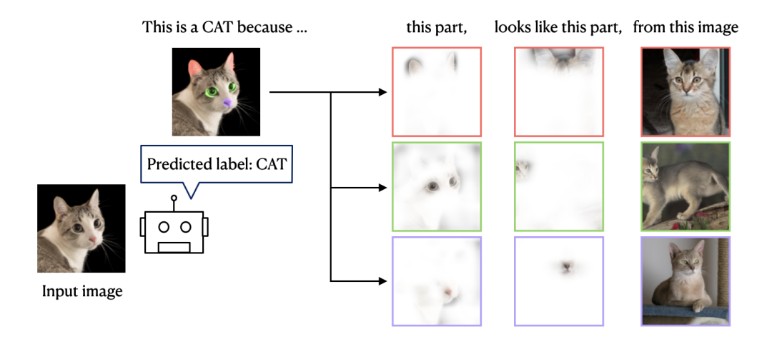
Part Prototype networks (e.g., ProtoPNet) are a family of models that incorporate interpretability right into the learning process. Rather than tacking interpretability on at the end, ProtoPNet learns prototypical parts and uses them to classify new inputs.
Architecture
Consider a simplified pipeline:
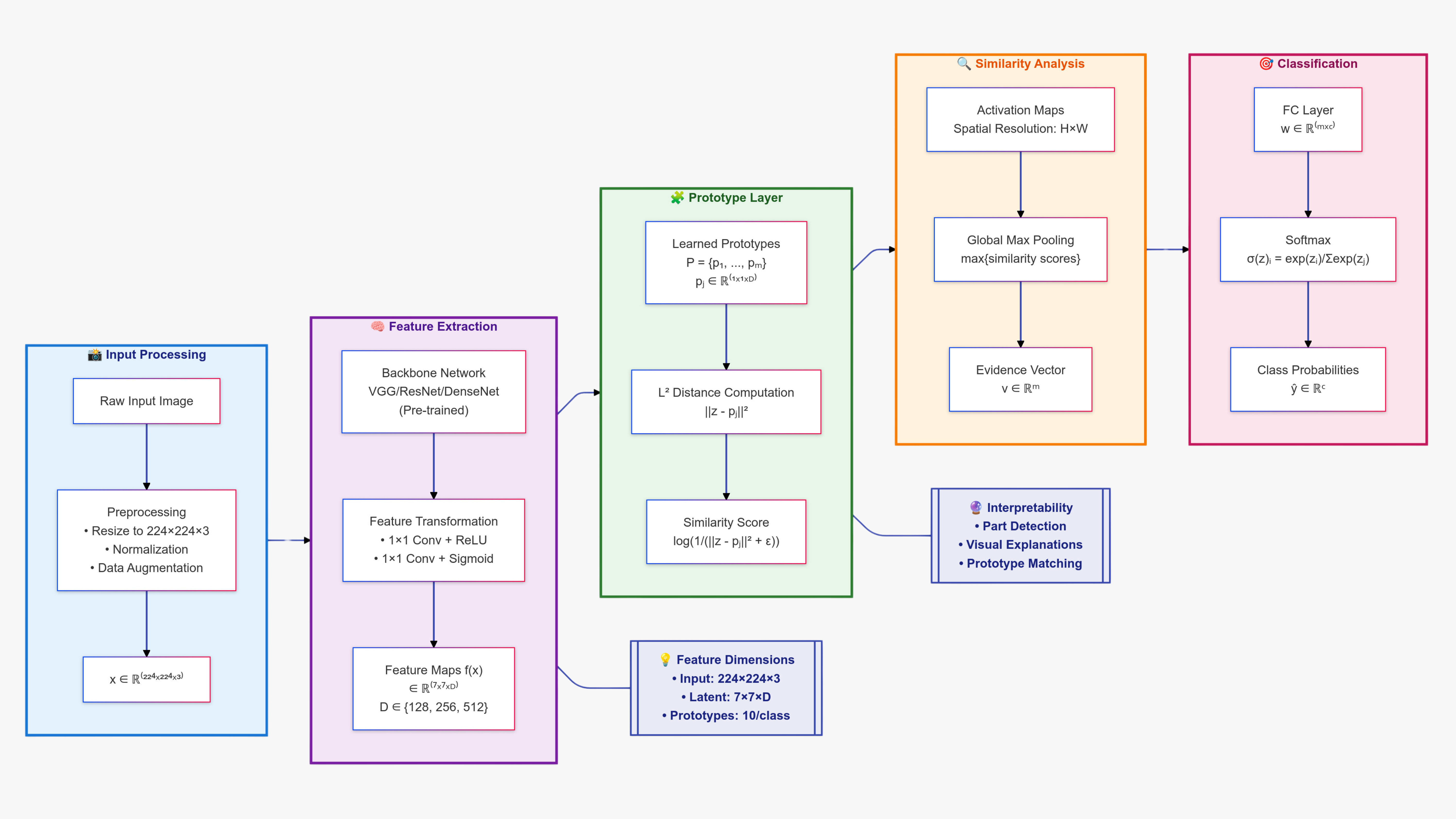
- Convolutional Layers: Extract feature maps from your input (e.g., an image).
- Prototype Layer: Stores one or more learned prototypes (these are also in a feature-space form).
- Similarity Computation: Compares the input's feature map to each prototype (often using $\ell_2$ distance).
- Fully Connected Layer: Aggregates those similarity scores to produce a class prediction.
Conceptually:
- If your input strongly resembles the "cat ear prototype," the similarity score is high for that prototype.
- High similarities for a bunch of "cat-like" prototypes boost the model's confidence in "cat."
Training Stages
Training typically happens in three main steps:
Stochastic Gradient Descent (SGD)
- Updates both the convolutional layers and the prototype representations to classify correctly.
Parameters Being Updated:
- Convolutional layers: Extract features from input images.
- Prototypes (P): Represent key parts of different classes.
Weight Initialization:
Initialize the weights $w_h^{(k,j)}$ which connect prototype $p_j$ to class $k$ as follows:
For Prototypes of Class $k$: $$w_h^{(k,j)} = 1, \quad \text{if } p_j \in P_k$$ Meaning: A prototype $p_j$ belonging to class $k$ will positively contribute to the class $k$ logic.
For Prototypes Not of Class $k$: $$w_h^{(k,j)} = -0.5, \quad \text{if } p_j \not\in P_k$$ Meaning: A prototype $p_j$ not belonging to class $k$ will negatively contribute to the class $k$ logic.
$$\min_{P,W_{conv}} \frac{1}{n} \sum_{i=1}^n \text{CrsEnt}(h \circ g_p \circ f(x_i), y_i) + \lambda_1\text{Clst} + \lambda_2\text{Sep}$$
where:
- Cross-Entropy Loss ($\text{CrsEnt}$): Penalizes incorrect classification.
- Clustering Loss ($\text{Clst}$): $$\text{Clst} = \frac{1}{n} \sum_{i=1}^n \min_{j:p_j \in P_{y_i}} \min_{z \in \text{patches}(f(x_i))} |z - p_j|^2$$ Encourages each image to have at least one patch close to a prototype of its class.
- Separation Loss ($\text{Sep}$): $$\text{Sep} = -\frac{1}{n} \sum_{i=1}^n \min_{j:p_j \not\in P_{y_i}} \min_{z \in \text{patches}(f(x_i))} |z - p_j|^2$$ Ensures patches are far from prototypes of other classes.
Prototype Projection
- Each prototype is snapped (or "projected") to the patch in the training set that most closely matches it. This ensures prototypes correspond to real examples, enhancing interpretability. $$p_j \leftarrow \arg\min_{z \in Z_j} |z - p_j|^2$$
where $Z_j = {z : z \in \text{patches}(f(x_i)) \text{ for } y_i = k}$ represents all patches from training images of the prototype's class.
Convex Optimization of the Last Layer
- Fine-tunes the classification weights for better accuracy and often improved interpretability.
$$\min_{w_h} \frac{1}{n} \sum_{i=1}^n \text{CrsEnt}(h \circ g_p \circ f(x_i), y_i) + \lambda \sum_{k=1}^K \sum_{j:p_j \not\in P_k} |w_h^{(k,j)}|$$
where the Sparsity Penalty ($|w_h^{(k,j)}|$) reduces reliance on negative reasoning (e.g., "This is not class $k$ because it doesn't match prototypes of $k$").
This optimization improves accuracy without changing the latent space or prototypes, encouraging the model to rely more on positive matches rather than negative ones.
Hardware note: Training can be resource-intensive. Something like 2×A100 GPUs or 3–4×V100 GPUs is typically recommended.
Comparison with Baseline Models
ProtoPNet often achieves competitive accuracy (within ~3.5% of the best big neural networks available) but offers a clear advantage in interpretability. Rather than just a final label, you see:
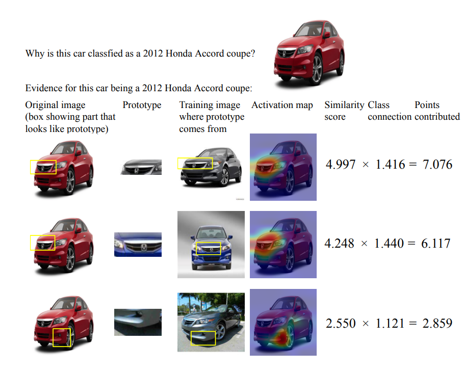
- Which prototypes fired.
- Why they fired (visual similarity).
- How confident the model is.
It's akin to case-based reasoning: "Here's the reference chunk from the training set, and here's your new input chunk. Look how similar they are!"
Shortcomings & Challenges
As cool as prototype networks are, they're not perfect. Here are a few known issues:
Spatial Rigidity
Prototypes often assume objects have fixed positions or orientations. If your image or object is rotated or partially out of the frame, the prototype might not match well.Semantic Mismatches
Occasionally, prototypes lock onto weird or irrelevant features (like the background rather than the object).
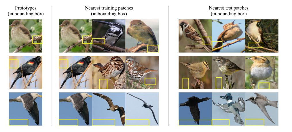
Limited Expressiveness
Sometimes the model learns redundant prototypes or fails to cover the full diversity of a class.Sensitivity to Transforms
Rotations, scalings, or small shifts can trip up the matching process, hurting performance.Occlusions & Partial Views
If part of the object is blocked, the prototype might not find a good match.Local Perturbation Noise
Small, local changes (like adding a bit of noise or a small sticker to an image) can throw off prototype matching.
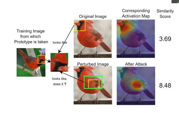
Despite these limitations, the transparency of part prototype networks often makes them a compelling option especially in safety-critical or user-facing scenarios.
Conclusion
Part Prototype networks (like ProtoPNet) offer a baked-in approach to interpretability. Instead of analyzing the model's decisions after the fact, the model learns prototypical parts right from the start. This can give users a more intuitive understanding of why the model made a certain call.
Still, no method is perfect:
- Post-hoc techniques remain valuable for any general model.
- Part Prototype-based networks provide a direct, case-based explanation but can limit flexibility.
As the field evolves, we might see more hybrid approaches or improved architectures that combine the clarity of prototypes with the versatility of large, powerful neural networks.
Additional Note: Theoretical Guarantees
An important theoretical result about ProtoPNet's projection step provides formal guarantees about prediction stability. Specifically:
- Stability Theorem: For correctly classified images, the prototype projection step maintains predictions under two conditions:
- Distance Bound: Prototypes don't move far from their pre-projection positions: $$\theta |z_i^k - b_i^k|_2 < \sqrt{c}$$
- Confidence Margin: The logit difference between the correct class and other classes exceeds a threshold: $$2\Delta_{max}$$
This means that when an image is correctly classified with sufficient confidence before projection, the projection step won't change its prediction. This theoretical foundation helps explain why ProtoPNet remains reliable even after prototype projection.
The computational efficiency is also worth noting:
- The prototype layer's cost is comparable to a standard convolutional layer with global pooling
- This makes it practical for real-world applications
- No significant overhead is added to the model's performance
Citation
Cited as:
Transformer, Vi. (Jan 2025). "Discussing ProtoPNet". 16x16 Words of Wisdom. https://vitransformer.netlify.app/posts/discussing-protopnet/
Or
@article{vit2025protopnet,
  title   = "Discussing ProtoPNet",
  author  = "Transformer, Vi",
  journal = "16x16 Words of Wisdom",
  year    = "2025",
  month   = "Jan",
  url     = "https://vitransformer.netlify.app/posts/discussing-protopnet/"
}
References
- Chen, C., Li, O., Tao, C., Barnett, A. J., Su, J., & Rudin, C. (2019). This Looks Like That: Deep Learning for Interpretable Image Recognition. arXiv preprint arXiv:1806.10574. https://arxiv.org/abs/1806.10574
- Hoffmann, A., Fanconi, C., Rade, R., & Kohler, J. (2021). This Looks Like That... Does it? Shortcomings of Latent Space Prototype Interpretability in Deep Networks. arXiv preprint arXiv:2105.02968. https://arxiv.org/abs/2105.02968
- P, J. J., Palanisamy, K., Chao, Y. W., Du, X., & Xiang, Y. (2024). Proto-CLIP: Vision-Language Prototypical Network for Few-Shot Learning. arXiv preprint arXiv:2307.03073. https://arxiv.org/abs/2307.03073
- Sivaprasad, S., Kangin, D., Angelov, P., & Fritz, M. (2025). COMIX: Compositional Explanations using Prototypes. arXiv preprint arXiv:2501.06059. https://arxiv.org/abs/2501.06059