Encoder + Explanatory Decoder

Making Foundational Models Explainable

Why do we need this model instead of just using other Prototype Networks?

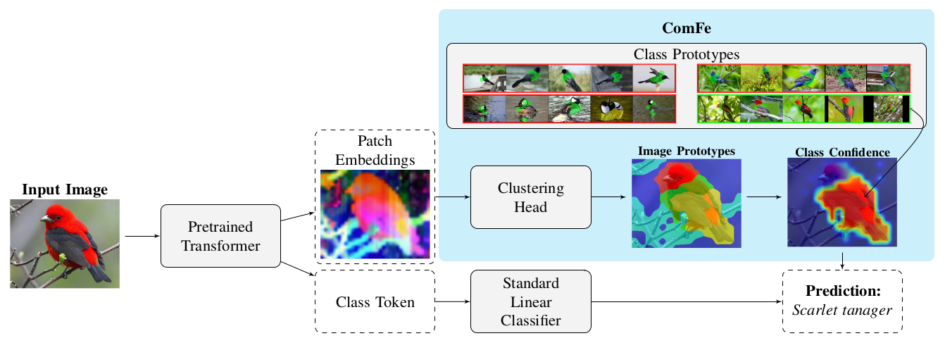
ComFe is the first interpretable approach that can scale to ImageNet-1K while being modular and efficient, requiring only a single GPU to train. Most importantly, it can obtain competitive performance in comparison to comparable non-interpretable methods.

More importantly, It is a new way to make Foundational Models explainable without retraining the backbone model. ComFe stands for Component Features hence it identifies like three most important parts of the image for the decision.
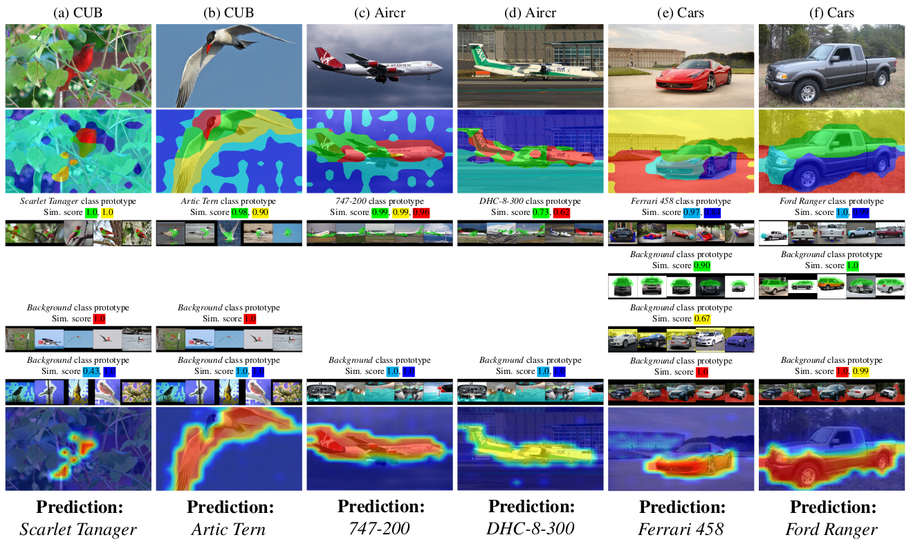
Example: Birds have a head, wings, body and background (3 more prototypes for just the background).

While traditional approaches solely rely on CLS tokens for classification, ComFe takes a different path. Instead of just using a single token for the entire image, it leverages both patch embeddings, image prototypes and class prototypes to provide interpretable predictions with localized explanations.

ComFe vs Non-interpretable Linear Classifier

👉 For background on prototype networks → Discussing ProtoPNet

👉 For background on ViT with prototypes → Vision Transformers Meet Prototypical Parts

Building Blocks

Before diving into ComFe, let's understand the foundation it builds upon.

DINOv2: The Foundation

DINOv2 is a state-of-the-art self-supervised learning framework. It creates rich visual representations without requiring any labels, through several key innovations:

Teacher-Student Architecture:
- Teacher processes weakly augmented images
- Student handles strongly augmented versions
- Weights updated via exponential moving average (EMA)

\[\theta_{teacher} = \lambda \cdot \theta_{teacher}^{prev} + (1-\lambda) \cdot \theta_{student}\]

Feature Space Properties:
- Semantic Consistency: Similar objects cluster together
- Scale Invariance: Robust to image size variations
- Directional Semantics: Linear directions encode meaningful attributes
Why DINOv2 for ComFe?:
- Rich patch embeddings (768D for ViT-B, 1024D for ViT-L)
- Frozen backbone requiring no fine-tuning
- Dense spatial understanding perfect for prototype learning
- Superior to CLIP for tasks requiring part understanding

The ComFe Framework: A New Approach

Building on DINOv2's powerful features, ComFe introduces a unique approach to interpretable vision models.

ComFe Architecture Overview: From Input to Interpretable Predictions

Core Components

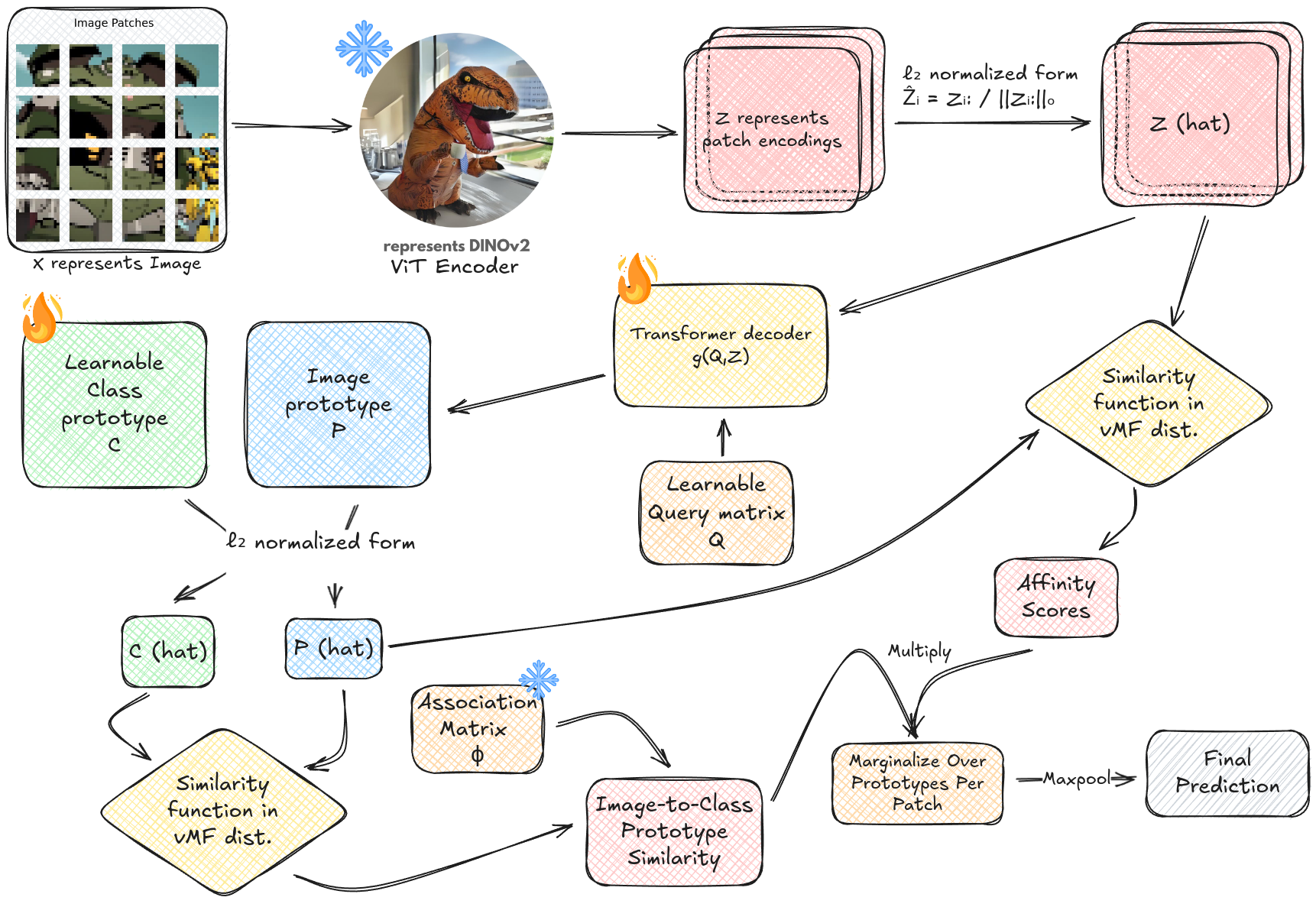
At its heart, ComFe transforms images into understandable decisions through three main stages:

Backbone

The process begins with DINOv2's Vision Transformer, which:

Divides input images into 16×16 pixel patches
Processes patches through multiple transformer layers
Generates rich semantic embeddings (768D for ViT-B, 1024D for ViT-L)

Prototype Learning

Think of prototypes as visual words describing the image. Just like we use words to describe what we see, ComFe uses prototypes to break down images into understandable components.

👉 For background on prototypes → Prototype Networks: What & Why?

Note: In ComFe, what we call "prototypes" are actually prototypical parts - smaller, localized features rather than whole-image prototypes. This aligns with how humans recognize objects through their distinctive parts.

The model uses a sophisticated prototype system:

Image-Specific Prototypes:
- Fixed set of 5 prototypes per image ($N_P = 5$)
- Transformer decoder maps normalized patches ($\hat{Z}$) to prototypes using learnable query matrix ($Q$)
- Each prototype captures a distinct component (e.g., "head", "wings", "body", "background")

Why 5 prototypes? This design choice balances granularity and computational efficiency. Fewer prototypes might miss important details, while more could add redundancy. Five prototypes work well empirically for complex datasets like ImageNet-1K.

Class Prototypes:
- Learned dictionary of class-specific features ($C$) during backpropagation
- Each class has 6 prototypes:
  - Prototypes 1-3: Class-specific features (e.g., distinctive parts of a bird)
  - Prototypes 4-6: Background features
- Association matrix ($\phi$) pre-assigns prototypes to classes:
  - Strongly links first 3 prototypes to their specific class
  - Weakly links last 3 prototypes for background features
- This design ensures prototypes naturally evolve to represent meaningful class features during training

Decisions Process

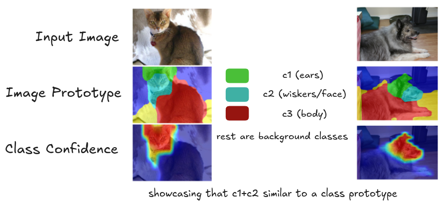
Visual breakdown of ComFe's clustering head

1. Image-to-Class Comparison

ComFe begins by comparing image prototypes against its library of class prototypes. Using vMF distribution as an inspiration leading to cosine similarity with temperature scaling and softmax, it identifies potential matches with high precision.

2. Prototype-Class Association

The association matrix ($\phi$) acts as a structured rulebook, creating strong links between prototypes and their primary classes while maintaining flexible connections to others. This ensures each prototype contributes meaningfully to classification while avoiding overly rigid assignments.

3. Local Feature Analysis

Each image patch embedding is analyzed for its relationship to image prototypes. We allow a patch to partially match multiple prototypes, capturing subtle visual relationships that might be crucial for classification.

4. Evidence Aggregation

ComFe weighs two key factors for each patch:

How well it matches each image prototype
How strongly those prototypes connect to different classes

This creates a sophisticated voting system where each patch's evidence is carefully weighted.

5. Final Decision

Rather than averaging all evidence, ComFe uses max-pooling to identify the strongest signals. A single distinctive feature (like a unique beak shape) can drive classification, even if most patches show only background elements.

Note on Normalization: L2 normalization projects all vectors (patch embeddings and prototypes) onto a unit hypersphere. This is crucial because it allows us to use the von Mises-Fisher (vMF) distribution, which is designed for directional data on unit hyperspheres. The vMF distribution provides a way to model the similarity between normalized vectors in high-dimensional spaces.

Probabilistic Foundation & Modeling

1. The Big Picture: Hierarchical Structure

ComFe uses a hierarchical mixture model to capture the relationships between normalized embeddings and prototypes:

\[p(\hat{Z}, \hat{P}, \nu) = p(\hat{Z}|\hat{P})p(\hat{P}|\nu)p(\nu)\]

This decomposition flows as:

\[\nu \rightarrow \hat{P} \rightarrow \hat{Z} \rightarrow \hat{y}\]

where:

$\hat{Z}$: normalized patch embeddings from DINOv2
$\hat{P}$: normalized image prototypes
$\nu$: class assignments
$p(\nu)$: Prior knowledge about class distribution
$\hat{y}$: Final predicted class

2. How It Works

a) Matching Patches to Prototypes

\[p(\hat{Z}_i|\hat{P}_j) \propto \exp\left(\frac{\hat{Z}_i \cdot \hat{P}_j}{\tau_1}\right)\]

Think of this as: "How well does this patch match this prototype?"

If a patch shows whiskers, it will have high similarity with the "whiskers" prototype
$\tau_1 = 0.1$ controls how strict the matching is

b) Connecting Prototypes to Classes

\[p(\hat{P}_j|\nu) \propto \sum_{l=1}^{N_C} \phi_{l,\nu} \cdot \exp\left(\frac{\hat{P}_j \cdot \hat{C}_l}{\tau_2}\right)\]

Think of this as: "How strongly does this prototype suggest a particular class?"

The association matrix $\phi$ acts like a rulebook:
- Strong connection ($\phi_{l,\nu} = 0.9$): "This prototype belongs to this class"
- Weak connection ($\phi_{l,\nu} = 0.001$): "This prototype might appear in other classes"
$\tau_2 = 0.02$ makes the model more certain about its choices

c) Making the Final Decision using Bayesian Inference

First, combine evidence for each patch:

\[p(\nu|\hat{Z}_i) = \sum_{j=1}^{N_P} p(\nu|\hat{P}_j) \cdot p(\hat{P}_j|\hat{Z}_i)\]

Then, make the final prediction:

\[p(y=l|X) = \max_i p(\nu=l|\hat{Z}_i)\]

Think of this as: "What's the strongest piece of evidence we have?"

If any patch is very confident about a class, that's our prediction
Example: A clear view of whiskers might be enough to say "cat"

Model Overview

1. Patch Embeddings

The input image $X \in \mathbb{R}^{3 \times H \times W}$ is processed by DINOv2 to produce patch embeddings, where:

\[Z = f(X) \in \mathbb{R}^{N_Z \times d}, \quad N_Z = \frac{H}{p} \times \frac{W}{p}\]

where:

$Z$: Output patch embeddings from DINOv2
$f(X)$: DINOv2 backbone function
$N_Z$: Number of patches (height × width)
$d$: Embedding dimension (768 for ViT-B, 1024 for ViT-L)
$p$: Patch size

These embeddings are L2-normalized:

\[\hat{Z}_{i:} = \frac{Z_{i:}}{\|Z_{i:}\|_2} \quad \forall i \in \{1, ..., N_Z\}\]

2. Prototype Generation

Image prototypes are generated using a transformer decoder with learnable queries and then normalized:

\[P = g_\theta(Q, \hat{Z}) \in \mathbb{R}^{N_P \times d}\]

\[\hat{P}_{j:} = \frac{P_{j:}}{\|P_{j:}\|_2} \quad \forall j \in \{1, ..., N_P\}\]

where:

$P$: Generated prototypes before normalization
$g_\theta$: Transformer decoder with parameters θ
$Q$: Learnable query matrix $\in \mathbb{R}^{N_P \times d}$
$N_P$: Number of prototypes per image (set to 5)
$\hat{P}_{j:}$: Normalized j-th prototype

3. Similarity Computations

Two key similarity measures are used with normalized vectors:

Patch-to-Prototype Affinity:

\[A_{ij} = \frac{\hat{Z}_{i:} \cdot \hat{P}_{j:}^T}{\tau_1}, \quad \tau_1 = 0.1\]

where:

$A_{ij}$: Affinity score between patch i and prototype j
$\tau_1$: Temperature parameter for scaling (0.1)
$\cdot$: Dot product operation

Prototype-to-Class Similarity:

\[S_{jk} = \frac{\hat{P}_{j:} \cdot \hat{C}_{k:}^T}{\tau_2}, \quad \tau_2 = 0.02\]

where:

$S_{jk}$: Similarity score between prototype j and class k
$\hat{C}_{k:}$: Normalized class prototype k
$\tau_2$: Temperature parameter for scaling (0.02)

4. Output Prediction Logic

The final prediction involves three key probability computations:

Class Relevance per Image Prototype:

\[p(\nu = l | \hat{P}_j) = \sum_{k=1}^{N_C} \phi_{k,l} \cdot \text{softmax}(S_j)_k\]

where:

$\phi_{k,l}$: Association strength between class k (predicted class) and l (actual class)
$N_C$: Number of classes

Patch-to-Prototype Assignment:

\[p(\hat{P}_j | \hat{Z}_i) = \text{softmax}(A_i)_j\]

Class Probability per Patch:

\[p(\nu = l | \hat{Z}_i) = \sum_{j=1}^{N_P} p(\nu = l | \hat{P}_j) \cdot p(\hat{P}_j | \hat{Z}_i)\]

The final prediction uses max-pooling over patches:

\[\hat{y} = \arg\max_l \max_i p(\nu = l | \hat{Z}_i)\]

where:

$\hat{y}$: Final predicted class

5. Loss Function

The total loss in ComFe combines three main components: clustering, discriminative classification, and auxiliary constraints. Let's break down each part:

1. Clustering Loss ($L_{\text{cluster}}$)

\[ L_{\text{cluster}}(\hat{Z};\, \theta,\mathbf{Q}) \;=\; - \frac{1}{N_z} \sum_{i=1}^{N_z}\; \log \;p(\hat{Z}_i) \;=\; -\frac{1}{N_z}\sum_{i=1}^{N_z}\sum_{j=1}^{N_p}\;\log \,k\bigl(\hat{Z}_i,\hat{P}_j;\tau_1\bigr)\;+\;C \]

where:

$\hat{Z}_i$: The normalized embedding of the $i$-th image patch
$\theta$: Parameters of the transformer decoder
$\mathbf{Q}$: Learnable query matrix for prototype generation
$N_z$: Total number of patches in the image
$N_p$: Number of prototypes per image (set to 5)
$k(\cdot,\cdot;\tau_1)$: Similarity function with temperature $\tau_1$
$\hat{P}_j$: The $j$-th normalized image prototype
$C$: Constant term resulting from the uniform prior

This loss ensures each patch is well-explained by the mixture of image prototypes. Think of it as forcing each patch to "fit" into at least one prototype. Without this, prototypes might not correspond to any real image parts!

Key Intuition: The model learns to group patches into local "components" (like heads, wings, backgrounds).

2. Discriminative Loss ($L_{\text{discrim}}$) [Just a BCE loss]

\[ L_{\text{discrim}}(Z, y; \theta, \mathbf{Q}, \mathbf{C}) \;=\; -\sum_{l=1}^c \bigl[ y_l \,\log\,p(y_l \mid \hat{Z}) \;+\; (1 - y_l)\,\log\bigl(1 - p(y_l \mid \hat{Z})\bigr) \bigr] \]

where:

$Z$: Raw patch embeddings from the backbone
$y_l$: Binary indicator (1 if class $l$ is present, 0 otherwise)
$c$: Total number of classes
$\mathbf{C}$: Learnable class prototypes
$p(y_l \mid \hat{Z})$: Probability of class $l$ given the normalized patches

This ensures correct classification at the image level. While we focus on local parts, we still need the final global label to be right. The classification uses aggregated signals from prototypes and so if something is labeled as a "Scarlet Tanager" then at least one prototype should strongly indicate that class.

3. Auxiliary Losses ($L_{\text{aux}}$)

These shape how prototypes behave, with three key components:

a) Prototype-Level Discriminative Loss

\[ L_{p\text{-discrim}}(Z,\,y;\,\theta,\mathbf{Q}) \;=\; -\sum_{l=1}^{c} \Bigl[ y_l\,\log\,p\bigl(y_l\mid \hat{P}\bigr) \;+\; (1 - y_l)\,\log\bigl(1 - p(y_l\mid \hat{P})\bigr) \Bigr] \]

Ensures that for each true class, at least one prototype yields high probability for that class. This prevents all prototypes from becoming background or unclassifiable.

b) Prototype Diversity Loss

\[ L_{\text{contrast}}(Z;\theta,\mathbf{Q},\mathbf{C}) = -\sum_{j=1}^{N_c} \log \frac{\exp(\hat{\mathbf{C}}_j \,\cdot\, \hat{\mathbf{C}}_j / \tau_c)} {\sum_{j'}\exp(\hat{\mathbf{C}}_{j'} \,\cdot\, \hat{\mathbf{C}}_j / \tau_c)} \;-\; \sum_{i=1}^{N_p} \log \frac{\exp(\hat{\mathbf{P}}_i \,\cdot\, \hat{\mathbf{P}}_i / \tau_c)} {\sum_{i'}\exp(\hat{\mathbf{P}}_{i'} \,\cdot\, \hat{\mathbf{P}}_i / \tau_c)} \]

where:

$N_c$: Number of class prototypes
$\tau_c$: Temperature parameter for contrast computation
$\hat{\mathbf{C}}_j$: The $j$-th normalized class prototype
$\hat{\mathbf{P}}_i$: The $i$-th normalized image prototype

This contrastive loss prevents prototypes from collapsing into identical embeddings. Each prototype must represent a distinct concept or part.

c) Consistency (CARL) Loss

\[ L_{\text{CARL}}(Z;\theta,\mathbf{Q}) \;=\; -\frac{1}{N_z}\sum_{i=1}^{N_z}\sum_{j=1}^{N_p} \;\log\,p\bigl(\hat{\mathbf{P}_j};\,\hat{Z}_i\bigr)\,p(\hat{\mathbf{P}_j}^{*\!};\,\hat{Z}_i^{*\!}) \]

where:

$\hat{Z}_i^*$: Normalized embedding of patch $i$ from an augmented view
$\hat{\mathbf{P}_j}^*$: Normalized Image prototype $j$ computed on the augmented view

Makes prototypes stable under data augmentations. If a patch matches a prototype in one view, it should match the same prototype even if the image is slightly modified.

The final objective combines all these components:

\[ L(Z,\,y; \theta,\mathbf{Q},\mathbf{C}) \;=\; L_{\text{cluster}} \;+\; L_{\text{discrim}} \;+\; L_{\text{aux}} \]

where $L_{\text{aux}} = L_{p\text{-discrim}} + L_{\text{contrast}} + L_{\text{CARL}}$

Note: While this might seem complex, each loss serves a specific purpose: clustering organizes patches, discrimination ensures correct classification, and auxiliary losses refine prototype behavior.

6. Association Matrix and Label Smoothing

The association matrix $\phi$ plays a crucial role in connecting prototypes to classes. Instead of using hard assignments, ComFe employs label smoothing to make the associations more flexible:

\[ \phi_{k,l} \,=\, \begin{cases} 1 - \alpha + \dfrac{\alpha}{c}, &\text{ if }(k \mod \tfrac{N_c}{c})=l,\\[6pt] \dfrac{\alpha}{c}, &\text{ otherwise.} \end{cases} \]

where:

$\phi_{k,l}$: Association strength between class prototype $k$ and class $l$
$\alpha$: Label smoothing parameter (typically small, e.g., 0.1)
$c$: Number of classes
$N_c$: Total number of class prototypes

This formulation means:

If prototype $k$ is meant to represent class $l$, its association strength is high but not exactly 1
For all other classes, it maintains a small non-zero association ($\frac{\alpha}{c}$)
The total association strengths for each prototype sum to 1

Takeaway: Label smoothing prevents prototypes from becoming too rigid in their class assignments, allowing them to capture shared visual patterns between similar classes while still maintaining clear primary associations.

Results

Performance comparison with other interpretable methods across different datasets

Non-interpretable Performance Comparison

Comparison against non-interpretable methods, showing competitive performance

Training efficiency comparison showing ComFe's computational advantages

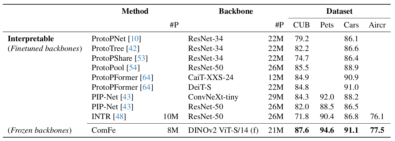
Hardware Note: All measurements were conducted on an NVIDIA A100 GPU (80GB) using a batch size of 64 on the CUB200 dataset.

Interpretability in Action: Visual Examples

Detailed visualization of ComFe explaining an image and its decisions

Visualization of class confidence heatmaps showing Informative regions randomly selected from some dataset

Citation

If you use this blog post, please cite it as:

Transformer, Vi. (Feb 2025). "Encoder + Explanatory Decoder". 16x16 Words of Wisdom. https://vitransformer.netlify.app/posts/encoder-explanatory-decoder/

@article{vit2025protovit,
  title   = "Encoder + Explanatory Decoder",
  author  = "Transformer, Vi",
  journal = "16x16 Words of Wisdom",
  year    = "2025",
  month   = "Feb",
  url     = "https://vitransformer.netlify.app/posts/encoder-explanatory-decoder/"
}

References

Mannix, E. J., Hodgkinson, L., & Bondell, H. (2024). ComFe: Interpretable Image Classifiers With Foundation Models. arXiv preprint arXiv:2403.04125. https://arxiv.org/abs/2403.04125
Oquab, M., Darcet, T., Moutakanni, T., Vo, H. V., Szafraniec, M., Khalidov, V., ... & Mairal, J. (2023). DINOv2: Learning Robust Visual Features without Supervision. arXiv preprint arXiv:2304.07193. https://arxiv.org/abs/2304.07193

Encoder + Explanatory Decoder

Making Foundational Models Explainable