Introduction
Vision Transformers have revolutionized computer vision. But like many deep learning models, they often lack interpretability. ProtoViT bridges this gap by combining:
- Vision Transformer's power (self-attention and patch-based processing)
- Prototype Network's interpretability (learning from recognizable examples)
👉 For background on prototype networks → Discussing ProtoPNet
A Quick Refresh
Before diving into ProtoViT, let's revisit the core ideas behind Vision Transformers (ViT):
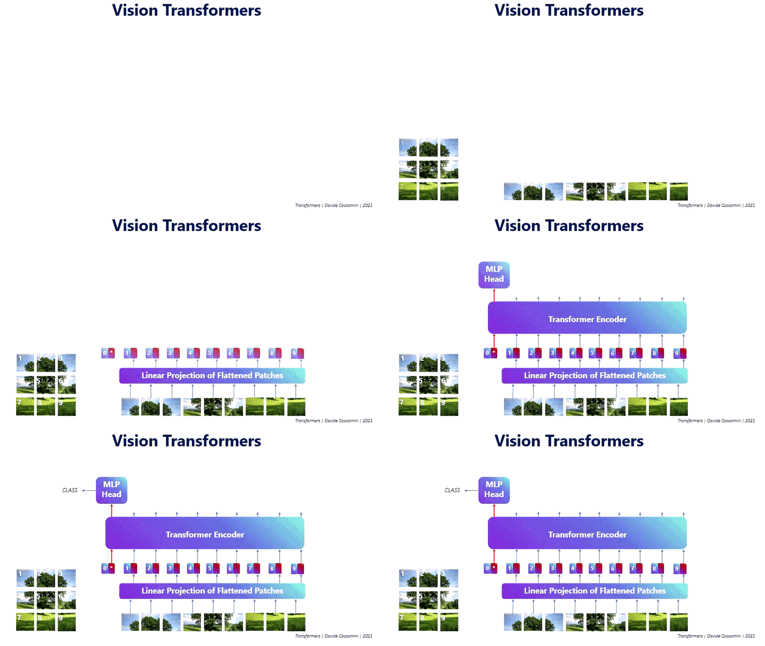
Patch-based Processing
Images are split into fixed-size patches (e.g., 16x16 pixels). These patches are flattened and linearly embedded, turning visual data into a sequence of "tokens".Position Embeddings
Unlike CNNs, ViTs have no inherent spatial awareness. Position embeddings are added to preserve spatial relationships between patches.Self-Attention Layers
Multiple transformer layers learn global relationships between patches. Each layer weighs the relevance of one patch to another, enabling dynamic feature learning.MLP Head for Classification
After processing through transformer blocks, a final MLP (Multilayer Perceptron) head generates class predictions.
Takeaway: ViTs replace convolutional layers with a pure transformer architecture, treating images as sequences and leveraging attention for long-range dependencies.
ProtoViT: The Best of Both Worlds
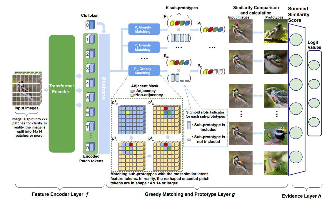
ProtoViT combines Vision Transformers with prototypical parts learning. Key innovations include:
- Transformer-based feature extraction
- Greedy matching and Sigmoid-based slots
- Interpretable decision process
Architecture Deep Dive
1. Vision Transformer Backbone
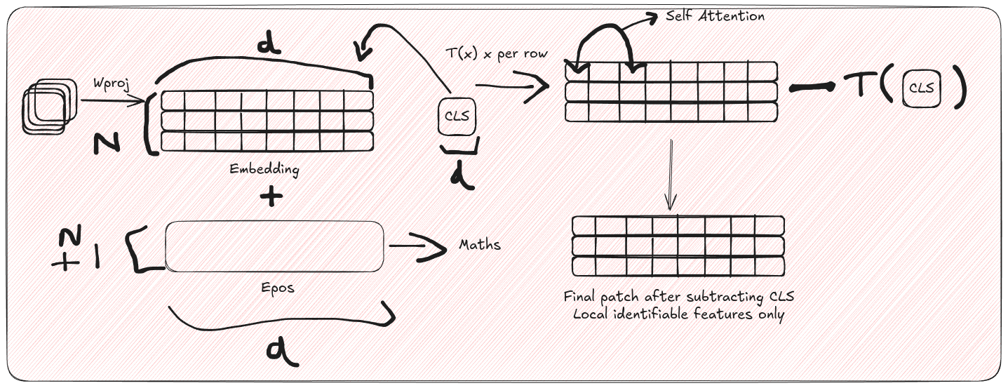
Input Processing:
- Images are split into patches (14×14 pixels)
- Each patch is flattened and linearly projected into a d-dimensional embedding space (d=768)
- Position embeddings are added to maintain spatial information
ViT Backbone:
- Standard transformer layers process the sequence of patch embeddings
- A learnable [CLS] token is prepended to patch embeddings
- Multi-head self-attention layers (12 heads) capture global relationships
Salient Feature Extraction:
# Highlighting distinctive local features
patch_features = patch_tokens - cls_token.expand_as(patch_tokens)
This can be written mathematically as:
$z_f = [z^1_f, z^2_f, \cdots, z^N_f]$, where $z^i_f = z^i_{patch} - z_{class}$, and $z^i_f \in \mathbb{R}^d$
2. Greedy matching and Prototype Layers
This layer is the heart of ProtoViT's interpretability. It enables the model to make explainable predictions by comparing input images with learned prototypes - key visual patterns that represent meaningful parts of objects.
At its core, ProtoViT learns a set of m prototypes, each composed of K sub-prototypes that represent different aspects of a visual concept. For example, a bird's beak prototype might have sub-prototypes for its tip, middle, and base. Mathematically, we represent this as:
$P = {p_1, p_2, ..., p_m}$
where each prototype $p_j = [p^1_j, p^2_j, ..., p^K_j]$
The layer works by matching these sub-prototypes to the most similar patches in the input image. This matching process uses cosine similarity to measure how well each image patch aligns with a sub-prototype:
$cos(z^i_f, p^k_j) = \frac{z^i_f \cdot p^k_j}{||z^i_f|| \cdot ||p^k_j||}$
Note: Unlike ProtoPNet which uses L2 distance, ProtoViT opts for cosine similarity. This choice makes the matching process more robust to variations in feature magnitudes, focusing instead on the directional alignment of feature vectors.
To ensure the matches make visual sense, the layer employs two key mechanisms:
Adjacency Masking ensures that matched patches are spatially close to each other. This prevents the model from matching disconnected parts of the image to the same prototype. For instance, when identifying a bird's beak, all matched patches should be near each other.
Adaptive Slots dynamically determine which sub-prototypes are important for the current image. Each sub-prototype gets an importance score that determines whether it should be included:
$\tilde{1}_{{\text{include }p^k_j}} = \text{Sigmoid}(v^k_j, \tau)$
The adaptive slots mechanism dynamically determines which sub-prototypes to include when computing prototype similarities. Let's break down its components:
- The indicator function $\tilde{1}_{{\text{include }p^k_j}} $ determines whether to include the $k$-th sub-prototype of prototype $j$.
- It uses a learnable parameter $\mathbf{v}_{j}^{k}$ that represents the importance of each sub-prototype.
- The temperature parameter $\tau$ controls the sharpness of the decision boundary through the sigmoid function.
For example, given a bird's beak prototype with three sub-prototypes (tip, middle, base), the mechanism might learn:
- High $\mathbf{v}_{j}^{k}$ for the tip ($\text{Sigmoid}(5.0, \tau) \approx 1$)
- Moderate for the middle ($\text{Sigmoid}(2.0, \tau) \approx 1$)
- Low for the base ($\text{Sigmoid}(-1.0, \tau) \approx 0$)
This allows the model to focus on the most relevant parts (tip and middle) while ignoring less important ones (base), making the similarity computation more precise and interpretable.
The final similarity score combines all these elements, weighing the contribution of each matched sub-prototype by its importance:

Let's understand the intuition behind this formula:
- Rescaling Factor ($\frac{K}{\sum \tilde{1}}$): This ensures prototypes with fewer included sub-prototypes aren't unfairly penalized. For instance, if only 2 out of 3 sub-prototypes of a bird's beak are visible in a side view, the similarity score is scaled by $\frac{3}{2}$ to maintain fair comparison.
This mechanism allows ProtoViT to break down its decisions into interpretable steps. When classifying a bird image, it might tell us:
"I see a bird because I found a beak-like pattern here (showing the matched patches), wing features there, and tail features over there."
3. Evidence layer
The Evidence Layer is the final component that converts prototype similarity scores into class predictions. It takes the similarity scores $g_{p_j}^{greedy}(z_f)$ from the Greedy matching and Prototype Layers and processes them through a fully connected layer making the final prediction which is interpretable through the prototype activations.
Training Process:
👉 For background on prototype network training, see Discussing ProtoPNet: Training Stages
1. Optimization of layers before last layer
The first phase optimizes all layers except the last one using SGD, with the goal of learning a latent space where feature patches naturally cluster near semantically relevant prototypes of their class. During initialization, all slot indicators $ \tilde{1}_{{\text{include }p^k_j}} $ are set to 1, and the last layer weights are initialized to connect each prototype to its corresponding class.
The training uses four specialized loss functions:
$L_{total} = L_{CE} + \lambda_1L_{Clst} + \lambda_2L_{Sep} + \lambda_3L_{Coh} + \lambda_4L_{Orth}$
Cross-Entropy Loss ($L_{CE}$): Standard classification loss that measures how well the model predicts the correct class:
Cluster Loss ($L_{Clst}$): Ensures each training image has features close to at least one sub-prototype of its class:
where:
$P_{y_i}$ is the set of prototypes belonging to the true class of image $i$
$p^k_j$ is the $k$-th sub-prototype of prototype $j$
$z^i_f$ is a feature token from image $i$
$z_{A^k_j}$ is the set of feature tokens in the adjacency region of the $k$-th sub-prototype
Separation Loss ($L_{Sep}$): Pushes features away from prototypes of incorrect classes:
where:
$p_j \notin P_{y_i}$ indicates prototypes not belonging to the true class of image $i$
Coherence Loss ($L_{Coh}$): Makes sub-prototypes within the same prototype semantically similar:
where:
$m$ is the number of prototypes
$p^k_j, p^s_j$ are pairs of sub-prototypes within prototype $j$ not the same prototype
$\tilde{1}$ is the indicator function determining sub-prototype inclusion
Orthogonality Loss ($L_{Orth}$): Promotes diversity and learns distinctive features among prototypes of the same class:
where:
- $C$ is the number of classes
- $P^{(l)}$ represents all prototypes belonging to class $l$, where each prototype is flattened into a single row vector of dimension $Kd$ (K sub-prototypes × d-dimensional features)
- $I_\rho$ is the identity matrix
- $|\cdot|_F$ denotes the Frobenius norm, which measures how far $P^{(l)}P^{(l)T}$ deviates from the identity matrix, effectively quantifying how orthogonal (dissimilar) the prototypes are to each other
2. Slots Pruning
The second phase focuses on removing sub-prototypes that don't align semantically with others in the same prototype. This pruning process ensures each prototype maintains a coherent visual concept.
Key Aspects:
- All model parameters are frozen except for slot indicators $\mathbf{v}^k_j$
- Uses a simplified loss function:
where $\lambda_5$ is intentionally reduced to prevent over-aggressive pruning.
The slot indicators are approximated using a sigmoid function with high temperature $\tau$, pushing values closer to binary decisions (0 or 1). After training completes, these values are rounded to create a definitive binary mask for each sub-prototype.
3. Prototype Projection
This phase anchors prototypes to real image patches, making them directly interpretable. The process involves:
Steps:
- Slot indicators are frozen with $\tilde{1}_{{\text{include }p^k_j}} = 0$ permanently excluding those sub-prototypes
- Each remaining prototype $p_j$ is projected onto the closest training image patch in the latent space using cosine similarity
- Thanks to ViT's patch-based architecture, these prototypes can be visualized directly without any upsampling
Theoretical Guarantee: If prototypes are well-trained (showing minimal movement during projection), the model's performance remains stable after projection. This guarantee comes from ProtoPNet's theoretical foundations.
4. Optimization of the Last Layer
This final phase optimizes the classification layer to enhance sparsity and interpretability while maintaining performance.
Procedure:
- Only the last layer weights $h$ are trained through convex optimization
- All other parameters remain frozen
- Uses a specialized loss function combining cross-entropy with L1 regularization:
where:
- $W_{b,l}$ represents weights connecting prototypes of class $l$ to output class $b$ (where $b \neq l$)
- $|W_{b,l}|_1$ is the L1 norm promoting sparsity
- $\lambda_6$ controls the strength of the sparsity penalty
The L1 penalty encourages the model to use only the most relevant prototypes for each class prediction, enhancing interpretability.
This staged training approach carefully balances model performance with interpretability, resulting in prototypes that are both discriminative and semantically meaningful.
Hardware Note: While ProtoPNet typically requires multiple high-end GPUs (2×A100 or 3-4×V100), ProtoViT can train on a single high-memory GPU:
- 1× NVIDIA Quadro RTX 6000 (24GB) or
- 1× NVIDIA GeForce RTX 4090 (24GB) or
- 1× NVIDIA RTX A6000 (48GB)
Comparison with Baseline

Advantages Over Traditional Approaches
For a technical comparison with other prototype-based approaches:
| Model | Support ViT Backbone? | Deformable Prototypes? | Coherent Prototypes? | Adaptive Sizes? | Inherently Interpretable? |
|---|---|---|---|---|---|
| ProtoPNet | Yes | No | Maybe | No | Yes |
| Deformable ProtoPNet | No | Yes | No | No | Yes |
| ProtoPformer | Yes | No | Maybe | No | No |
| ProtoViT | Yes | Yes | Yes | Yes | Yes |
Comparison of Different Model Backbones
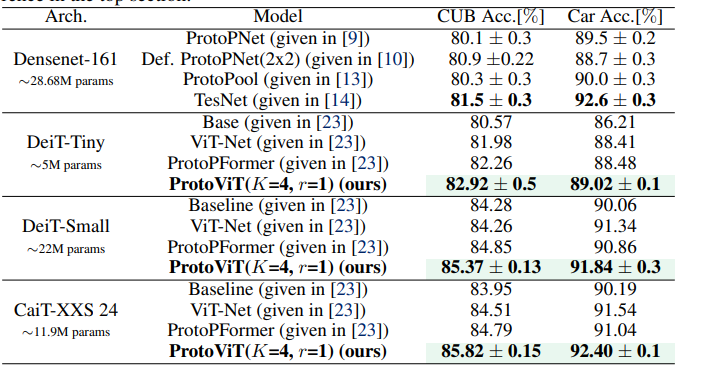
Results and Visualizations
Analysis: ProtoPNet vs ProtoVit

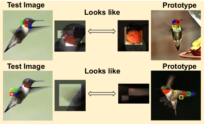
Classification Examples


Limitations
Explainability Gaps
- Lacks textual explanations for its reasoning
- Requires domain-specific vocabularies for specialized fields
- Visual explanations may not align with human-interpretable concepts without post-hoc analysis
Technical Challenges
- Location misalignment in deeper layers
- Resolution constraints (optimal at 224×224 pixels)
- Performance degradation with domain shifts
Data Dependencies
- Training bias from specific datasets
- Limited generalization to dissimilar domains
- Prototype interpretability varies with data quality
Implementation Resources
Official Implementation
The original implementation is available on GitHub:
ProtoViT Official Repository
Community Implementation
An improved fork with dockerfile and preprocessing scripts:
ProtoViT Enhanced Fork
Pre-trained Models
CUB-200-2011 Dataset
- Model: DeiT-Small
- 🤗 Download Weights
Pinterest Face Recognition Dataset
- Model: DeiT-Small
- 🤗 Download Weights
Citation
Cited as:
Transformer, Vi. (Feb 2025). "Vision Transformers Meet Prototypical Parts". 16x16 Words of Wisdom. https://vitransformer.netlify.app/posts/vision-transformers-meet-prototypical-parts/
Or
@article{vit2025protovit,
  title   = "Vision Transformers Meet Prototypical Parts",
  author  = "Transformer, Vi",
  journal = "16x16 Words of Wisdom",
  year    = "2025",
  month   = "Feb",
  url     = "https://vitransformer.netlify.app/posts/vision-transformers-meet-prototypical-parts/"
}
References
- Dosovitskiy, A., Beyer, L., Kolesnikov, A., Weissenborn, D., Zhai, X., Unterthiner, T., ... & Houlsby, N. (2021). An Image is Worth 16x16 Words: Transformers for Image Recognition at Scale. arXiv preprint arXiv:2010.11929. https://arxiv.org/abs/2010.11929
- Chen, C., Li, O., Tao, C., Barnett, A. J., Su, J., & Rudin, C. (2019). This Looks Like That: Deep Learning for Interpretable Image Recognition. arXiv preprint arXiv:1806.10574. https://arxiv.org/abs/1806.10574
- Ma, C., Donnelly, J., Liu, W., Vosoughi, S., Rudin, C., & Chen, C. (2024). Interpretable Image Classification with Adaptive Prototype-based Vision Transformers. arXiv preprint arXiv:2410.20722. https://arxiv.org/abs/2410.20722